Introduction
This lecture talks about methods that optimise policy directly. Instead of working with value function as we consider so far, we seek experience and use the experience to update our policy in the direction that makes it better.
In the last lecture, we approximated the value or action-value function using parameters \(\theta\), \[ V_\theta(s)\approx V^\pi(s)\\ Q_\theta(s, a)\approx Q^\pi(s, a) \] A policy was generated directly from the value function using \(\epsilon\)-greedy.
In this lecture we will directly parametrise the policy \[ \pi_\theta(s, a)=\mathbb{P}[a|s, \theta] \] We will focus again on \(\color{red}{\mbox{model-free}}\) reinforcement learning.
Table of Contents
- Finite Difference Policy Gradient
- Monte-Carlo Policy Gradient
- Actor-Critic Policy Gradient
- Summary of Policy Gradient Algorithms
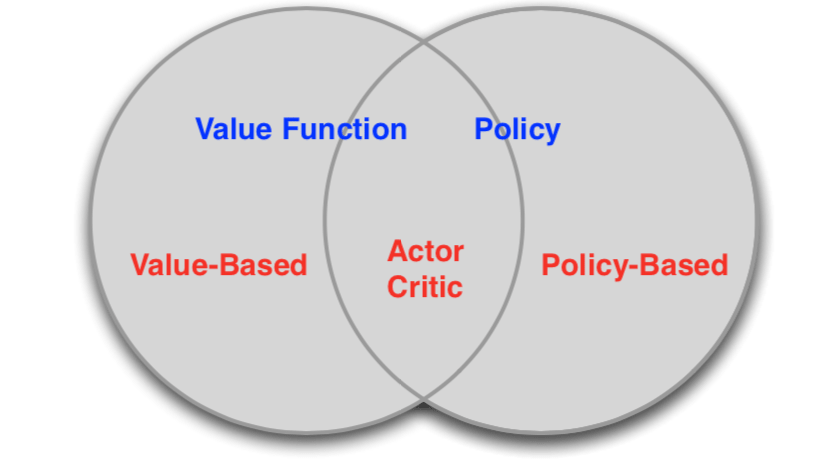
Value-Based and Policy-Based RL
- Value Based
- Learnt Value Function
- Implicit policy (e.g. \(\epsilon\)-greedy)
- Policy Based
- No Value Function
- Learnt Policy
- Actor-Critic
- Learnt Value Function
- Learnt Policy
Advantages of Policy-Based RL
Advantages:
- Better convergence properties
- Effective in high-dimensional or contimuous action spaces (without computing max)
- Can learn stochastic policies
Disadvantages:
- Typically converge to a local rather than global optimum
- Evaluating a policy is typically inefficient and high variance
Deterministic policy or taking max is not also the best. Take the rock-paper-scissors game for example.

Consider policies iterated rock-paper-scissors
- A deterministic policy is easily exploited
- A uniform random policy is optimal (according to Nash equilibrium)
Aliased Gridworld Example

The agent cannot differentiate the grey states.
Consider features of the following form (for all N, E, S, W) \[ \phi(s, a)=1(\mbox{wall to N, a = move E}) \] Compare value-based RL, using an approximate value function \[ Q_\theta(s, a)=f(\phi(s, a), \theta) \] To policy-based RL, using a parametrised policy \[ \pi_\theta(s, a)=g(\phi(s, a), \theta) \] Since the agent cannot differentiate the grey states given the feature, if you take a deterministic policy, you must pick the same action at two grey states.

Under aliasing, an optimal \(\color{red}{\mbox{deterministic}}\) policy will either
- move W in both grey states (as shown by red arrows)
- move E in both grey states
Either way, it can get stuck and never reach the money.
Value-based RL learns a near-deterministic policy, so it will traverse the corridor for a long time.

An optimal \(\color{red}{\mbox{stochastic}}\) policy will randomly move E or W in grey states: \[ \pi_\theta(\mbox{wall to N and S, move E}) = 0.5\\ \pi_\theta(\mbox{wall to N and S, move W}) = 0.5\\ \] It will reach the goal state in a few steps with high probability. Policy-based RL can learn the optimal stochastic policy.
These examples show that a stochastic policy can be better than the deterministic policy, especially in the case that the MDP is partialy observed or cannot fully represent the state.
Policy Objective Functions
Goal: given policy \(\pi_\theta(s, a)\) with parameters \(\theta\), find best \(\theta\). But how do we measure the quality of a policy \(\pi_\theta\)?
In episodic environments we can use the start value \[ J_1(\theta)=V^{\pi_\theta}(s_1)=\mathbb{E}_{\pi_\theta}[v_1] \]
In continuing environments we can use the average value \[ J_{av}v(\theta)=\sum_s d^{\pi_\theta}(s)V^{\pi_\theta}(s) \]
Or the average reward per time-step
\[ J_{av}R(\theta)=\sum_s d^{\pi_\theta}(s)\sum_a\pi_\theta(s, a)\mathcal{R}^a_s \]
where \(d^{\pi_\theta}(s)\) is stationary distribution of Markov chain for \(\pi_\theta\).
Policy Optimisation
Policy based reinforcement learning is an optimisation problem. Find \(\theta\) that maximises \(J(\theta)\).
Some approaches do not use gradient
- Hill climbing
- Simplex / amoeba / Nelder Mead
- Genetic algorithms
However, greater efficiency often possible using gradient
- Gradient descent
- Conjugate gradient
- Quasi-newton
We focus on gradient descent, many extensions possible. And on methods that exploit sequential structure.
Finite Difference Policy Gradient
Policy Gradient
Let \(J(\theta)\) be any policy objective function. Policy gradient algorithms search for a local maximum in \(J(\theta)\) by ascending the gradient of the policy, w.r.t. parameters \(\theta\) \[ \triangle\theta = \alpha\nabla_\theta J(\theta) \] Where \(\bigtriangledown_\theta J(\theta)\) is the \(\color{red}{\mbox{policy gradient}}\), \[ \nabla_\theta J(\theta)=\begin{pmatrix} \frac{\partial J(\theta)}{\partial \theta_1} \\ \vdots\\ \frac{\partial J(\theta)}{\partial \theta_n} \end{pmatrix} \] and \(\alpha\) is a step-size parameter.
Computing Gradients By Finite Differences (Numerical)
To evaluate policy gradient of \(\pi_\theta(s, a)\).
- For each dimension \(k\in[1, n]\):
Estimate \(k\)th partial derivative of objective function w.r.t. \(\theta\)
By perturbing \(\theta\) by small amount \(\epsilon\) in \(k\)th dimension \[ \frac{\partial J(\theta)}{\partial \theta_k}\approx \frac{J(\theta+\epsilon u_k)-J(\theta)}{\epsilon} \] where \(u_k\) is unit vector with 1 in \(k\)th component, 0 elsewhere
- Uses \(n\) evaluations to compute policy gradient in \(n\) dimensions
This is a simple, noisy, inefficient, but sometimes effective method. It works for arbitrary policies, even if policy is not differentiable.
The algorithm is efficient when the dimension of \(\theta\) is low.
Monte-Carlo Policy Gradient
Score Function
We now compute the policy gradient analytically.
Assume policy \(\pi_\theta\) is differentiable whenever it is non-zero and we know the gradient \(\nabla_\theta\pi_\theta(s, a)\).
\(\color{red}{\mbox{Likelihood ratios}}\) exploit the following identity \[ \begin{align} \nabla_\theta\pi_\theta(s, a) & =\pi_\theta(s, a) \frac{\nabla_\theta\pi_\theta(s, a) }{\pi_\theta(s, a) } \\ & = \pi_\theta(s, a) \nabla_\theta\log \pi_\theta(s, a) \\ \end{align} \] The \(\color{red}{\mbox{score function}}\) is $(s, a) $. Let's take two examples to see what the score function looks like.
Softmax Policy
We will use a softmax policy as a running example. Weight actions using linear combination of features \(\phi(s, a)^T\theta\). Probability of action is proportional to exponentiated weight: \[ \pi_\theta(s, a)\varpropto e^{\phi(s, a)^T\theta} \] The score function is \[ \nabla_\theta\log\pi_\theta(s, a)=\phi(s, a)-\mathbb{E}_{\pi_\theta}[\phi(s, \cdot)] \] (Intuition: log gradient = the feature for the action that we actually took minus the average feature for all actions.)
Gaussian Policy
In continuous action spaces, a Gaussian policy is natural.
- Mean is a linear combination of state features \(\mu(s) = \phi(s)^T\theta\).
- Variance may be fixed \(\sigma^2\), or can also parametrised
Policy is Gaussian, \(a\sim \mathcal{N}(\mu(s), \sigma^2)\). The score function is \[ \nabla_\theta\log\pi_\theta(s, a)=\frac{(a-\mu(s))\phi(s)}{\sigma^2} \] So far we just have a sense of what does the score function look like. Now we step into policy gradient theorem.
One-Step MDPs
Consider a simple class of one-step MDPs:
- Starting in state \(s\sim d(s)\)
- Terminating after one time-step with reward \(r=\mathcal{R}_{s,a}\)
Use likelihood ratios to compute the policy gradient \[ \begin{align} J(\theta) &=\mathbb{E}_{\pi_\theta}[r]\\ &=\sum_{s\in\mathcal{S}}d(s)\sum_{a\in\mathcal{A}}\pi_\theta(s, a)\mathcal{R}_{s,a} \end{align} \]
\[ \begin{align} \nabla_\theta J(\theta) &=\sum_{s\in\mathcal{S}}d(s)\sum_{a\in\mathcal{A}}\pi_\theta(s, a)\nabla_\theta\log\pi_\theta(s, a)\mathcal{R}_{s,a}\\ &=\mathbb{E}_{\pi_\theta}[\nabla_\theta\log\pi_\theta(s, a)r] \end{align} \]
The policy gradient theorem generalises the likelihood ratio approach to multi-step MDPs.
- Replaces instantaneous reward \(r\) with long-term value \(Q^\pi(s, a)\)
Policy gradient theorem applies to start state objective, average reward, and average value objective.
Theorem
For any differentiable policy \(\pi_\theta(s,a)\), for any of the policy objective functions mentioned earlier, the policy gradient is \[ \nabla_\theta J(\theta)=\color{red}{\mathbb{E}_{\pi_\theta}[\nabla_\theta\log\pi_\theta(s, a)Q^{\pi_\theta}(s, a)]} \]
Demonstration
Settings: The initial state \(s_0\) is sampled from distribution \(\rho_0\). A trajectory \(\tau = (s_0, a_0, s_1, a_1, ..., s_{t+1})\) is sampled from policy \(\pi_\theta\).
The target function would be \[ J(\theta) = E_{\tau\sim\pi}[R(\tau)] \] The probability of trajectory \(\tau\) is sampled from \(\pi\) is \[ P(\tau|\theta) = \rho_0(s_0)+\prod_{t=0}^TP(s_{t+1}|s_t, a_t)\pi_\theta(a_t|s_t) \] Using the log prob trick: \[ \triangledown_\theta P(\tau|\theta) = P(\tau|\theta)\triangledown_\theta\log P(\tau|\theta) \] Expand the trajectory: \[ \begin{align} \require{cancel}\triangledown_\theta \log P(\tau|\theta) &= \cancel{\triangledown_\theta \log\rho_0(s_0)}+\sum_{t=0}^T\cancel{\triangledown_\theta \log P(s_{t+1}|s_t,a_t)}+ \triangledown_\theta\log\pi_\theta(a_t|s_t)\\ &= \sum_{t=0}^T\triangledown_\theta\log\pi_\theta(a_t|s_t) \end{align} \] The gradient of target function \[ \begin{align} \triangledown_\theta J(\theta) &= \triangledown_\theta E_{\tau\sim\pi}[R(\tau)]\\ &= \int_\tau \triangledown_\theta P(\tau|\theta)R(\tau)\\ &= \int_\tau P(\tau|\theta)\triangledown_\theta \log P(\tau|\theta)R(\tau)\\ &= E_{\tau\sim\pi}[\triangledown_\theta \log P(\tau|\theta)R(\tau)]\\ &= E_{\tau\sim\pi}[\sum_{t=0}^T\triangledown_\theta\log\pi_\theta(a_t|s_t)R(\tau)]\\ &= E_{\tau\sim\pi}[\sum_{t=0}^T \color{red}{\Phi_t}\triangledown_\theta\log\pi_\theta(a_t|s_t)] \end{align} \]
Monte-Carlo Policy Gradient (REINFORCE)
Update parameters by stochastic gradient ascent using policy gradient theorem. And using return \(v_t\) as an unbiased sample of \(Q^{\pi_\theta}(s_t,a_t)\): \[
\triangle\theta_t=\alpha\nabla_\theta\log\pi_\theta(s_t, a_t)v_t
\] 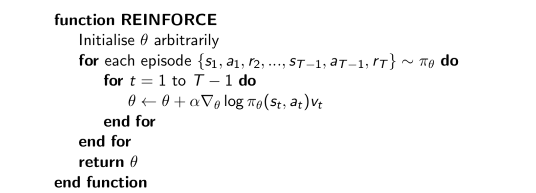
(Note: MCPG is slow.)
Actor-Critic Policy Gradient
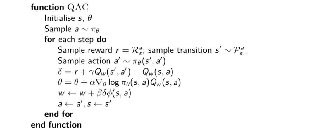
Reducing Variance Using a Critic
Monte-Carlo policy gradient still has high variance, we use a \(\color{red}{critic}\) to estimate the action-value function: \[ Q_w(s, a)\approx Q^{\pi_\theta}(s, a) \] Actor-critic algorithms maintain two sets of parameters:
- Critic: Updates action-value function parameters \(w\)
- Actor: Updates policy parameters \(\theta\), in direction suggested by critic
Actor-critic algorithms follow an approximate policy gradient: \[ \nabla_\theta J(\theta)\approx \mathbb{E}_{\pi_\theta}[\nabla_\theta\log\pi_\theta(s, a)Q_w(s, a)]\\ \triangle\theta= \alpha\nabla_\theta\log\pi_\theta(s, a)Q_w(s, a) \] The critic is solving a familiar problem: policy evaluation. This problem was explored in previous lectures:
- Monte-Carlo policy evaluation
- Temporal-Difference learning
- TD(\(\lambda\))
- Least Squares policy evaluation
Simple actor-critic algorithm based on action-value critic using linear value function approximation. \(Q_w(s, a)=\phi(s,a)^Tw\)
- Critic: Updates \(w\) by linear TD(0)
- Actor: Updates \(\theta\) by policy gradient
Bias in Actor-Critic Algorithms
Approximating the policy gradient introduces bias. A biased policy gradient may not find the right solution. Luckily, if we choose value function approximation carefully, then we can avoid introducing any bias. That is we can still follow the exact policy gradient.
Compatible Function Approximation Theorem
If the following two conditions are satisdied:
Value function approximator is compatible to the policy \[ \nabla_w Q_w(s, a)=\nabla_\theta \log\pi_\theta(s, a) \]
Value function parameters \(w\) minimise the mean-squared error \[ \epsilon=\mathbb{E}_{\pi_\theta}[(Q^{\pi_\theta}(s, a)-Q_w(s, a))^2] \]
Then the policy gradient is exact, \[ \nabla_\theta J(\theta)=\mathbb{E}_{\pi_\theta}[\nabla_\theta\log\pi_\theta(s,a)Q_w(s,a)] \]
Trick: Reducing Variance Using a Baseline
We substract a baseline function \(B(s)\) from the policy gradient. This can reduce variance, without changing expectation: \[ \begin{align} \mathbb{E}_{\pi_\theta}[\nabla_\theta\log\pi_\theta(s,a)B(s)]&=\sum_{s\in\mathcal{S}}d^{\pi_\theta}(s)\sum_a\nabla_\theta\pi_\theta(s,a)B(s)\\ &= \sum_{s\in\mathcal{S}}d^{\pi_\theta}B(s)\nabla_\theta\sum_{a\in\mathcal{A}}\pi_\theta(s,a)\\ &= \sum_{s\in\mathcal{S}}d^{\pi_\theta}B(s)\nabla_\theta 1 \\ &=0 \end{align} \] A good baseline is the state value function \(B(s)=V^{\pi_\theta}(s)\). So we can rewrite the policy gradient using the \(\color{red}{\mbox{advantage function}}\ A^{\pi_\theta}(s,a)\). \[ A^{\pi_\theta}(s,a)=Q^{\pi_\theta}(s,a)-V^{\pi_\theta}(s)\\ \nabla_\theta J(\theta)=\mathbb{E}_{\pi_\theta}[\nabla_\theta\log\pi_\theta(s,a)\color{red}{A^{\pi_\theta}(s,a)}] \] where \(V^{\pi_\theta}(s)\) is the state value function of \(s\).
Intuition: The advantage function \(A^{\pi_\theta}(s,a)\) tells us how much better than usual is it to take action \(a\).
Estimating the Advantage Function
How do we know the state value function \(V\)?
One way to do that is to estimate both \(V^{\pi_\theta}(s)\) and \(Q^{\pi_\theta}(s,a)\). Using two function approximators and two parameter vectors, \[ V_v(s)\approx V^{\pi_\theta}(s)\\ Q_w(s,a)\approx Q^{\pi_\theta}(s,a)\\ A(s,a)=Q_w(s,a)-V_v(s) \] And updating both value functions by e.g. TD learning.
Another way is to use the TD error to compute the policy gradient. For the true value function \(V^{\pi_\theta}(s)\), the TD error \(\delta^{\pi_\theta}\) \[ \delta^{\pi_\theta}=r+\gamma V^{\pi_\theta}(s')-V^{\pi_\theta}(s) \] is an unbiased estimate of the advantage function: \[ \begin{align} \mathbb{E}_{\pi_\theta}[\delta^{\pi_\theta}|s, a] &= \mathbb{E}_{\pi_\theta}[r+\gamma V^{\pi_\theta}(s')|s, a]-V^{\pi_\theta}(s)\\ &= Q^{\pi_\theta}(s, a) - V^{\pi_\theta}(s)\\ &= \color{red}{A^{\pi_\theta}(s,a)} \end{align} \] So we can use the TD error to compute the policy gradient \[ \nabla_\theta J(\theta)=\mathbb{E}_{\pi_\theta}[\nabla_\theta\log\pi_\theta(s,a)\color{red}{\delta^{\pi_\theta}}] \] In practice we can use an approximate TD error: \[ \delta_v=r+\gamma V_v(s')-V_v(s) \] This approach only requires one set of critic parameters \(v\).
Critics and Actors at Different Time-Scales
Critic can estimate value function \(V_\theta(s)\) from many targets at different time-scales
For MC, the target is return \(v_t\) \[ \triangle \theta=\alpha(\color{red}{v_t}-V_\theta(s))\phi(s) \]
For TD(0), the target is the TD target \(r+\gamma V(s')\) \[ \triangle \theta=\alpha(\color{red}{r+\gamma V(s')}-V_\theta(s))\phi(s) \]
For forward-view TD(\(\lambda\)), the target is the return \(_vt^\lambda\) \[ \triangle \theta=\alpha(\color{red}{v_t^\lambda}-V_\theta(s))\phi(s) \]
For backward-view TD(\(\lambda\)), we use eligibility traces \[ \begin{align} \delta_t &= r_{t+1}+\gamma V(s_{t+1})-V(s_t) \\ e_t& = \gamma\lambda e_{t-1} +\phi(s_t) \\ \triangle\theta&=\alpha\delta_te_t \end{align} \]
The policy gradient can also be estimated at many time-scales \[ \nabla_\theta J(\theta)=\mathbb{E}_{\pi_\theta}[\nabla_\theta\log\pi_\theta(s,a)\color{red}{A^{\pi_\theta}(s,a)}] \]
MC policy gradient uses error from complete return \[ \triangle\theta=\alpha(\color{red}{v_t}-V_v(s_t))\nabla_\theta\log\pi_\theta(s_t,a_t) \]
Actor-critic policy gradient uses the one-step TD error \[ \triangle\theta=\alpha(\color{red}{r+\gamma V_v(s_{t+1})}-V_v(s_t))\nabla_\theta\log\pi_\theta(s_t,a_t) \]
Just like forward-view TD(\(\lambda\)), we can mix over time-scale \[ \triangle \theta=\alpha(\color{red}{v_t^\lambda}-V_v(s_t))\nabla_\theta\log\pi_\theta(s_t,a_t) \] where \(v_t^\lambda-V_v(s_t)\) is a biased estimate of advantage function.
Like backward-view TD(\(\lambda\)), we can also use eligibility traces by substituting \(\phi(s)=\nabla_\theta\log\pi_\theta(s,a)\) \[ \begin{align} \delta_t &= r_{t+1}+\gamma V_v(s_{t+1})-V_v(s_t) \\ e_{t+1}& = \gamma\lambda e_{t} +\nabla_\theta\log\pi_\theta(s,a) \\ \triangle\theta&=\alpha\delta_te_t \end{align} \]
Summary of Policy Gradient Algorithms
The policy gradient has many equivalent forms
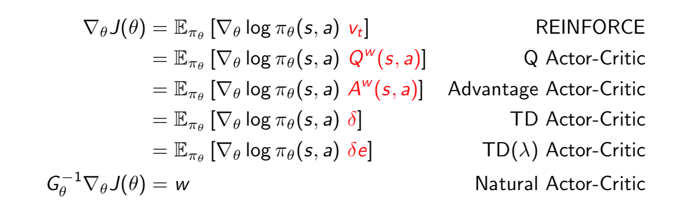
Each leads a stochastic gradient ascent algorithm. Critic uses policy evaluation to estimate \(Q^\pi(s, a)\), \(A^\pi(s, a)\) or \(V^\pi(s)\).